

Oleksandr Maksimeniuk, founder and CVO of Ringostat started his work with tables in his students years. That’s why people usually ask him how to write a formula or process data. According to his words, the most common mistake is difficult solutions for tasks that could be solved easier. Or when something that could be automated is done manually. Oleksandr has prepared a list of tips: from simple to difficult, for those who work with Google Sheets and wants to improve himself.
English interface and the United States location
In the English interface, a coma “,” is the function argument separator. Thus, all solutions that we will discuss below are customized for the coma. The locale also influences the decimal separator in numbers as in the English version it is the dot “.” However, you also need to remember that symbols that are used in Google Sheets’ functions are different for various languages.
Why the United States locale? There will definitely be dots, it is native and the most common — that’s why it has fewer bugs. Pay attention that the date there is presented in month/date/year form, and the separator is slash, as you can see.
Validation
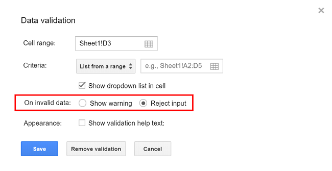
It is especially important when different employees manually enter data to the document, so it means that they can make mistakes. Validation sets in the following section: Data — Data Validation, and can be of two types:
- loose validation — there will appear a window with the message about the error if you enter data in a wrong format;
- strong validation — it is impossible to enter mistaken data.
Naming
Give the more clear name possible to the spreadsheet. Moreover, the name has to be clear not only for you but also for people who will receive access. Thus, you will avoid the situation when you need to find something and there are only “Untitled documents” on the list. The example of naming: “Report on the effectiveness of employees / Jones / November 2019 / N Company”.
We have a local joke. The document has to be named the way so you will find it by punching the keyboard at 4 AM after a party.
Design
- place numbers and money on the right border of the column, equally rounded and with the same separator between decimals — thus, you will easier find out numbers of another decimal;
- place the text on the left border — this makes reading easier;
- the date is in the middle;
- pin upper rows of the column if a document doesn’t fit a single screen;
- delete blank cells and columns using Crop Sheet — thus, you will be sure that there is no other data in the document that are simply not visible, and you won’t also reach the limit of 400 000 cells per sheet.
Tips described in this article may seem complicated. Especially if you are a business owner or a marketer who needs reports to understand the efficacy of the ad and the cost recovery of investments in it. In this case, a ready-made instrument — end-to-end analytics will suit you. It automatically brings the key data and counts the cost recovery of investments in the advertisement — ROI.
Work with formulas
Train yourself to make all calculations using formulas — even if you need to count 2+2. Calculated (dependent) values may be without formulas only in two cases:
- if you import prepared data from other sources;
- when there are too much data in the documents and it becomes “large” — you have to delete some of the formulas here so it will download faster.
Some simple tips for beginners
- Look at hints. They appear as soon as you start to enter the formula and the developed description appears when you click on the hint. There are described examples and designation of conditions and values.
- Create formulas using basic knowledge. It is not necessary to remember thousands of formulas — sometimes it is possible to “collect” what you need. For example, there is a document with the data on the blog — overall (general), English version (en). It is required to transpose an array (we will describe it below) by the general data only. Then the formula will be the following: =TRANSPOSE(FILTER(A1:X22,A1:А = “general”)). Where: A1:X22 — the whole; A1:A = blog_general — condition 1).
- Search for the prepared solution on Stack Overflow. There are solutions for most of the tasks and they are presented in several options. The optimal variant is often marked by a tick.
- Use F4 to faster change fixed references in formulas. If you select the relative reference and press this button for once, the $ symbol will automatically appear. However, take into account that this won’t work with mixed references — for example, $A1 or A$1, they are half relative and half absolute. Read more about the type of address in Google support.
Read the names of all formulas and their descriptions in the Google support.
Formula Modifiers
IF and IFS work for many functions but you need to remember at least the basic ones:
- SUM;
- AVERAGE — average value;
- COUNT — count of the number, for example, cells, symbols in a row, but not their contents.
If you add “IF” to these functions, there will be a verification of the one certain condition. But when “IFS” added, the amount of conditions is multiple. And values will be displayed only during their implementation.
One more useful formula is UNIQUE. It returns unique rows in the set range, meanwhile, deleting duplicates. There is a spreadsheet on the example below with sources and channels that have duplicated titles. It is required to calculate the number of sessions and the coefficient of the conversion for each of them. We need to sum data by each channel by doing so. For example, all sessions from google cpc. Our steps:
- choose unique values using UNIQUE;
- using SUMIF, set the condition that all values are summed if utm_source is google, and utm_medium is cpc;
- use $ to pin the rage.
ARRAYFORMULA
Displays values in several rows and columns received via the array formula. With its simplicity, it makes the work with Sheets much easier. Let’s say there is a large array of data that has to be processed — to count the conversion rate in the example below. We could split the value of one cell to another and extend it.
What is the advantage of ARRAYFORMULA:
- speed;
- the limit on the number of formulas is not wasted — we will describe it below;
- usefulness — enter rages, press Enter, so the formula counted and extended everything.
ARRAYFORMULA can be used for more complex tasks. Let’s say, you need to calculate the amount and make the verification by REGEX — accurate matching to a certain text. There is no formula that works with the array if you make the verification for compliance with the regular expression.
Imagine a document with the mentioned transfers from all sources. We are interested exactly in transfers from Facebook. Meanwhile, in the documents, there are five marks with the word Facebook (for example, Facebook_buisness) and three more with shortened Fb (Fb_123). Due to the type of this formula, REGEXMATCH, we can sum values that have mention of both words Facebook and Fb in the text.
It is possible to use ARRAYFORMULA with any other formulas, besides INDEX, SEARCH, QUERY, etc. SUM may also work incorrectly in some cases. When you select two or more arrays they have to be of the same size.
Another implementation of the ARRAYFORMULA is the data transfer from one sheet to another, staying in the same document. Let’s say, a dashboard is created in the document. It has 200 rows and 30 columns. We import data to a separate sheet in the same document and using ARRAYFORMULA, pull a huge rage — horizontally and vertically. For example, it is possible to pull 5 rows of data for three years, using a single formula.
Formulas that are important to remember
- IMPORTRANGE — allows importing a range of cells from a specified spreadsheet that you have access to.
- SPLIT — divides text around a specified character or string. For example, we have a document for prioritization calculation — features Ringostat. There is an ID of the task and its description from the system of project management, placed in one cell. We pull everything till space into the next cell — in other words, only ID. Additionally, there can be formed a reference (HYPERLINK formula) via the CONCATENATE formula.
- UNIQUE — Returns unique rows in the provided source range, discarding duplicates. The result is the array. You can insert a two-dimensional array in UNIQUE and choose unique rows in it.
- VLOOKUP and HLOOKUP — VLOOKUP searches down the first column of a range for a key and returns the value of a specified cell in the row found. HLOOKUP searches across the first row of a range for a key and returns the value of a specified cell in the column found. Let’s get back to the example from the 2nd paragraph. There is a document with ID, title and description of the feature, its score. The formula allows pulling the feature title by the list of keys.
- TRANSPOSE — transposes the rows and columns of an array or range of cells. Let’s say, there is an array with titles in the first row but we need to arrange them in a column. Thus, data that was placed from left to right are transposed to the column — from top to bottom. The rage can also be transposed via “paste special”.
- IF — is useful in cases when SUMIF and SUMIFS are not enough.
- SORT — sorts the rows of a given criterion. In the same document with the scoring calculation features, we pull a massive from another document. Firstly, we delete duplicates using UNIQUE and the sort by score.
Useful tips
- {A1:A20,C1:C20} {A1:A20;C1:C20} — give a single array, meanwhile, the result depends on a separator. Let’s get back once again to the example with the table for features prioritization. We are interested in columns A, B, and M. The thing is that it is impossible to import this rage and paste without columns — and consolidation of arrays doesn’t allow us to do so. However, both variants work with the US locale. The option with a coma provides a horizontal combining of arrays. The one with a semicolon will consolidate data in one column.
- A1&B1 — consolidates values from several rows in one. This one is also possible A1&” “&B1.
- “Some text” — text is framed by double-quotes. If, in case, you use apostrophes as “usual quotes”, consider that they are used for other goals in Google Sheets.
- Don’t forget to add =if(D2>20,true,) separator in the end, if you need to bring a blank row via FALSE result within IF function. Otherwise, you will receive FALSE.
- If the formula is put ahead and contains a division, NA/0 will be displayed instead of blank cells. To make it more “pretty” and make the cell blank, the formula is covered by IFERROR =iferror(ARRAYFORMULA(E2:E/D2:D)).
- CTRL(CMD — для Mac) + SHIFT + V — paste values. It is needed if you copy cells with formulas and want to simply paste a value. The formatting is as well deleting with the insertion.
- The row of formulas editing extends in height. To break lines during formulas creation or editing, CTRL(CMD) + Enter is used. The line break is not considered as a symbol. It is a much easier way to edit, especially when the formula is big.
- F2 on the cell opens its editing. This is super useful when you mostly use a keyboard and don’t want to “search for” the mouse.
- ≠ is written as <>. For example, if you need to find all values that are not equal to certain content. For example, google cpc.
- =sum(arrayformula(if(REGEXMATCH(C2:C10,”some regEx”),D2:D10,0))) — this has to be understood to open the third eye while working with Google Sheets 🙂 Oleksandr says that he has faced a lot of cases like that.
If the document is that large so it is not comfy to work in it
- Use more compact functions. For example, the QUERY is very large. Sure, it has more opportunities but in most cases, VLOOKUP is enough to complete the same goals.
- Decrease the number of IMPORTRANGE. During the data import from several documents, each time the file is rendering, the formula takes the data, pastes, counts, etc. Considering the load, it is rather easier to form a final sheet with all values for import in the first document. And create the same sheet in the second document and import there all the required data. As a result, data would be transported at once and the initial file wouldn’t be opened five times. Then this information can be placed on the sheets needed for work, for example, using ARRAYFORMULA.
- Use optimal solutions. Conclusions made from our own experience are useful there. For example, when there is a great amount of data =IFERROR(B1/A1) is “more compact” than =IF(B17<>0,C17/B17,).
- Go to the external data aggregation. Transfer them to the BigQuery or another database. You can process data there and import finished values to Google Sheets. Google Apps Script (GScript) is useful to do so.
- Delete formulas from cells that don’t have to be revised. For example, data older than three months. Use CTRL + C, and then CTRL + SHIFT + V for the same cells — a document has become “more compact”.
Limitations
- 5,000,000 cells, with a maximum of 256 columns per sheet;
- 40 000 cells that contain formulas;
- 200 sheets per one document;
- 1 000 GoogleFinance formulas;
- 1 000 GoogleLookup formulas;
- ImportRange: 50 formulas to import from other documents;
- 50 ImportData formulas, ImportHtml, ImportFeed or ImportXm.